

Network Reconstruction#
Network reconstruction is the process of inferring the structure of a network from time series data. This is a crucial step in understanding the relationships between different nodes in a complex system. Put simply, network reconstruction applies connectivity measures to each pair of time series. This results in a \((n \times n)\) matrix of \(p\)-values and lags.
The reconstruct_network() Function#
The delaynet package provides the
reconstruct_network() function to generate
\(p\)-value matrices by applying connectivity measures to pairs of time series.
As described in the Connectivity section, connectivity measures return
\(p\)-values that indicate the strength of connections between time series.
Therefore, the \(p\)-value matrix in network reconstruction represents a matrix of
\(p\)-values, where lower values indicate stronger connections.
Complete Network Reconstruction Example#
This comprehensive example demonstrates the entire workflow of network reconstruction, from data generation to network visualization and validation. We’ll use synthetic data with a known ground truth to evaluate the reconstruction performance.
Data Generation and Preprocessing#
First, we generate synthetic time series data using a delayed causal network (DCN) model. This approach creates time series with known causal relationships, allowing us to validate our reconstruction results.
Generated time series: (8, 1000)
Adjacency matrix: (8, 8)
Weight matrix: (8, 8)
The generated data contains 8 time series of length 1000, along with the true adjacency and weight matrices that define the underlying network structure. Before proceeding with network reconstruction, we apply detrending to remove trends and make the time series stationary.
Note that we use axis=1 in the detrending function because we have multiple time
series arranged as rows, and we want to detrend each time series individually across its
temporal dimension.
time_series = dn.detrend(time_series, "delta", axis=1)
print(f"Detrended time series: {time_series.shape}")
Detrended time series: (8, 1000)
Network Reconstruction#
Now we apply the reconstruct_network() function
to infer the network structure from the preprocessed time series data. We use Granger
causality as our connectivity measure, which is particularly well-suited for detecting
directed causal relationships in time series data.
# Reconstruct with Granger Casuality
weights, lags = dn.reconstruct_network(
    time_series.T, connectivity_measure="gc", lag_steps=10
)
Sequential: [##############################] 56/56 (100.0%) Time: 0.7s
Visualizing the Results#
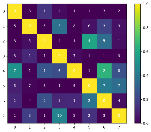
The reconstruction function returns two matrices: a \(p\)-value matrix indicating the strength of connections (lower values = stronger connections) and a lag matrix showing the optimal time delays. We visualize these results as a heatmap with the \(p\)-values as colors and the optimal lags as text annotations.
Network Pruning#
To convert the continuous \(p\)-value matrix into a binary adjacency matrix, we apply statistical thresholding. We use a significance level (α) of 0.02, meaning we only consider connections with \(p\)-values below this threshold as statistically significant. This pruning step is crucial for removing weak or spurious connections and focusing on the most reliable network edges.
# Prune weight matrix
pruned_weights = weights.copy()
threshold = 0.02  # Adjust threshold as needed
pruned_weights = 1 * (pruned_weights < threshold)
# pruned_weights = 1 - pruned_weights
# set diagonal to 0
pruned_weights[np.diag_indices_from(pruned_weights)] = 0
Validation Against Ground Truth#
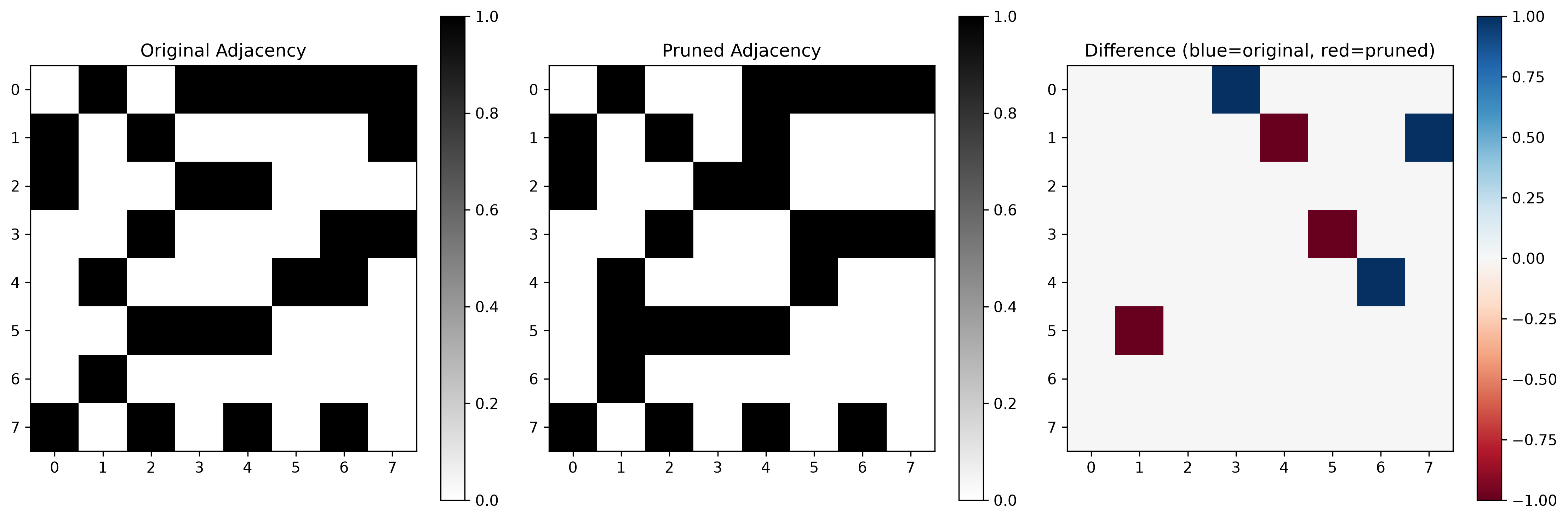
In real-world applications, the true network structure is typically unknown. However, since we used synthetic data, we can compare our reconstructed network against the ground truth adjacency matrix. This validation step helps us assess the accuracy of our reconstruction method.
The visualization shows three matrices: the original (ground truth) adjacency matrix, our reconstructed and pruned adjacency matrix, and their difference. In the difference plot, blue regions indicate edges that exist only in the original network (false negatives), while red regions show edges that were inferred but don’t exist in the true network (false positives).
Network Graph Visualization#
To better understand the reconstruction results, we create a network graph that visually distinguishes between different types of edges. This representation makes it easier to identify correctly reconstructed connections, missed connections, and false discoveries.
G = nx.from_numpy_array(adjacency_matrix, create_using=nx.DiGraph)
G_pruned = nx.from_numpy_array(pruned_weights, create_using=nx.DiGraph)
G_union = nx.compose(G, G_pruned)
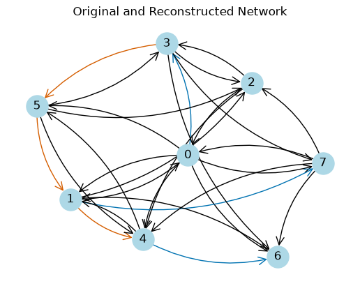
This example showed the reconstruction of a network from synthetic time series data with known ground truth, demonstrating the complete workflow from data generation through validation and providing a framework for evaluating reconstruction accuracy in controlled scenarios.
API Reference and Usage Examples#
Basic Usage#
import numpy as np
from delaynet.network_reconstruction import reconstruct_network

# Generate sample data: 100 time points, 5 nodes
np.random.seed(42)  # For reproducible results
data = np.random.randn(100, 5)

# Reconstruct network using linear correlation
weights, lags = reconstruct_network(data, "linear_correlation", lag_steps=5)

print(f"P-value matrix shape: {weights.shape}")
print(f"Lag matrix shape: {lags.shape}")
print(f"P-value matrix:\n{weights}")
print(f"Lag matrix:\n{lags}")
Sequential: [##############################] 20/20 (100.0%) Time: 0.0s
P-value matrix shape: (5, 5)
Lag matrix shape: (5, 5)
P-value matrix:
[[1.         0.14530612 0.67143519 0.14358786 0.01041288]
 [0.39814884 1.         0.09741699 0.33473627 0.1544949 ]
 [0.16127713 0.2775177  1.         0.45232073 0.27574542]
 [0.1985502  0.19202054 0.05616415 1.         0.04791115]
 [0.27173079 0.14710467 0.0526507  0.2395354  1.        ]]
Lag matrix:
[[0 3 4 2 2]
 [3 0 2 3 3]
 [5 1 0 3 2]
 [1 1 4 0 1]
 [3 2 3 4 0]]
Understanding the Output#
The function returns two matrices:
\(p\)-value Matrix: Contains \(p\)-values representing the strength of connections between nodes. Lower \(p\)-values indicate stronger connections.
Lag Matrix: Contains the optimal time lags at which the strongest connections were found.
# Analyze the results
print("Strong connections (p < 0.05):")
strong_connections = np.where(weights < 0.05)
for i, j in zip(strong_connections[0], strong_connections[1]):
    if i != j:
        print(f"Node {i} -> Node {j}: p-value = {weights[i,j]:.4f}, lag = {lags[i,j]}")
Strong connections (p < 0.05):
Node 0 -> Node 4: p-value = 0.0104, lag = 2
Node 3 -> Node 4: p-value = 0.0479, lag = 1
Using Different Connectivity Measures#
You can use any of the available connectivity measures:
# Using transfer entropy
weights_te, lags_te = reconstruct_network(data, "transfer_entropy", approach = "ksg", lag_steps=3)

# Using mutual information
weights_mi, lags_mi = reconstruct_network(data, "mutual_information", approach = "ksg", lag_steps=3)

print(f"Transfer entropy p-values:\n{weights_te}")
print(f"Mutual information p-values:\n{weights_mi}")
Sequential: [##############################] 20/20 (100.0%) Time: 1.1s
Sequential: [##############################] 20/20 (100.0%) Time: 2.0s
Transfer entropy p-values:
[[1.   0.5  0.05 0.2  0.  ]
 [0.6  1.   0.25 0.2  0.5 ]
 [0.2  0.3  1.   0.15 0.45]
 [0.65 0.   0.45 1.   0.45]
 [0.3  0.25 0.4  0.3  1.  ]]
Mutual information p-values:
[[1.   0.3  0.1  0.8  0.05]
 [0.2  1.   0.15 0.35 0.4 ]
 [0.3  0.25 1.   0.55 0.9 ]
 [0.95 0.35 0.45 1.   0.85]
 [0.   0.45 0.85 0.95 1.  ]]
Custom Connectivity Measures#
You can also provide your own connectivity measure as a callable:
def custom_correlation_metric(ts1, ts2, lag_steps=None):
    """Custom connectivity measure based on correlation."""
    # Simple example: return absolute correlation as p-value and lag 1
    correlation = abs(np.corrcoef(ts1, ts2)[0, 1])
    return correlation, 1  # not really a p-value and lag - for demonstration purposes

# Use custom metric
weights_custom, lags_custom = reconstruct_network(data, custom_correlation_metric, lag_steps=5)
print(f"Custom metric p-values:\n{weights_custom}")
Sequential: [##############################] 20/20 (100.0%) Time: 0.0s
Custom metric p-values:
[[1.         0.16343282 0.04486628 0.10183222 0.12618359]
 [0.16343282 1.         0.12276426 0.03821481 0.0571554 ]
 [0.04486628 0.12276426 1.         0.00852457 0.04281939]
 [0.10183222 0.03821481 0.00852457 1.         0.01835847]
 [0.12618359 0.0571554  0.04281939 0.01835847 1.        ]]
Function Reference#
- delaynet.network_reconstruction.reconstruct_network(time_series: ndarray, connectivity_measure: str | Callable[[ndarray, ndarray, ...], tuple[float, int]], lag_steps: int | list[int] | None = None, workers: int = None, **kwargs) tuple[ndarray, ndarray][source]#
Reconstruct a network from time series data.
This function applies a connectivity measure to all pairs of time series to construct a network represented by weight and lag matrices.
- Parameters:
time_series (numpy.ndarray) – Array of time series data with shape (n_time, n_nodes). Each column represents a time series for one node.
connectivity_measure (str or Callable) – Connectivity measure to use. Can be either a string name of a built-in measure or a callable function. Available string measures can be found using
delaynet.connectivity.show_connectivity_metrics(). If a callable is provided, it should take two time series as input and return a tuple of (float, int).lag_steps (int | list[int] | None) – The number of lag steps to consider. Required. Can be integer for [1, …, num], or a list of integers.
workers (int | None) – Number of workers to use for parallel computation.
kwargs (dict) – Additional keyword arguments passed to the connectivity measure.
- Returns:
Tuple containing:
weight_matrix: Matrix of p-values with shape (n_nodes, n_nodes). Lower p-values indicate stronger connections.
lag_matrix: Matrix of optimal time lags with shape (n_nodes, n_nodes).
- Return type:
- Raises:
ValueError – If time_series has incorrect dimensions.
ValueError – If
connectivity_measureis unknown (when given as string).ValueError – If
connectivity_measurereturns invalid value (when given as callable).ValueError – If
connectivity_measureis neither string nor callable.
Example:#
>>> import numpy as np
>>> from delaynet.network_reconstruction import reconstruct_network
>>> # Generate sample data: 100 time points, 5 nodes
>>> data = np.random.randn(100, 5)
>>>
>>> # Using string metric
>>> weights, lags = reconstruct_network(data, "linear_correlation", lag_steps=5)
>>> weights.shape
(5, 5)
>>> lags.shape
(5, 5)
>>>
>>> # Using callable metric
>>> def custom_metric(ts1, ts2, lag_steps=None):
...     # Using numpy cov function
...     all_values = [np.cov(ts1[: -lag or None], ts2[lag:])[0,1] for lag in lag_steps]
...     idx_optimal = min(range(len(all_values)), key=all_values.__getitem__)
...     return all_values[idx_optimal], lag_steps[idx_optimal]
>>> weights, lags = reconstruct_network(data, custom_metric, lag_steps=5)
>>> weights.shape
(5, 5)
Note:#
The diagonal elements of the weight matrix are set to 1.0 by default, indicating no significant self-connection.
Next Steps#
After reconstructing a network, the next step is typically to analyze its properties and extract meaningful insights. The Network Analysis section provides tools for pruning networks based on statistical significance and calculating various network metrics such as centrality measures, link density, and global efficiency.