Connectivity

delaynet provides a variety of connectivity measures to analyze the relationships between time series. These measures can be used to detect causal relationships, correlations, and synchronisation between different time series.

To measure a significant correlation between two time series, each connectivity approach calculates a \(p\)-value. This \(p\)-value indicates the probability that the observed correlation between two time series is due to random chance. A strong correlation results in a low \(p\)-value.

One assumption is that the information propagation in the network can have varying delays between each node in the network. Due to this, the connectivity needs to be calculated for different delay steps. It is possible to either test for all delays up to a certain maximum delay or to test for specific delays. The best delay value and it’s corresponding \(p\)-value are returned.

To visualise this, we generate synthetic time series data using a delayed causal network (DCN) model. The data consists of eight interconnected nodes with 1000 time points each, where causal relationships exist between different time series with varying delays. We extract two specific time series from this network and apply Granger causality to find the optimal lag that produces the strongest causal relationship. The algorithm tests all possible lags from 1 to 50 time steps and identifies the lag that yields the minimum p-value, indicating the most significant causal connection.

Show code cell source

Hide code cell source

import delaynet as dn
from delaynet.connectivities.granger import gt_single_lag
from numpy.random import default_rng
from matplotlib import pyplot as plt

_, _, time_series = dn.preparation.gen_delayed_causal_network(
    ts_len=1000,                # Length of time series
    n_nodes=8,                  # Number of nodes
    l_dens=0.8,                 # Density of the adjacency matrix
    wm_min_max=(0.5, 1.5),      # Min and max of the weight matrix
    rng=default_rng(1612956748129757)
)

# Extract two time series
ts1 = time_series[0]
ts2 = time_series[1]
max_lag = 50

# Using this package
best_p_value, lag = dn.connectivity(ts1, ts2, "gc", lag_steps=max_lag)

print(f"Best lag: {lag}")
print(f"Best p-value: {best_p_value}")

# Visualisation on how this value is found:
p_values = []
for lag in range(1, max_lag + 1):
    p_value = gt_single_lag(ts1, ts2, lag)
    p_values.append(p_value)

# Plotting the P-values
plt.figure(figsize=(10, 4), dpi = 300)
plt.plot(range(1, max_lag + 1), p_values, marker='o')
plt.axvline(x=p_values.index(min(p_values)) + 1, color='r', linestyle='--', label=f'Minimum P-value at lag {p_values.index(min(p_values)) + 1}')
plt.title(r'$p$-values for Different Lags in GC Connectivity')
plt.xlabel('Lag')
plt.ylabel('$p$-value')
plt.legend()
plt.grid(True)
plt.show()

Best lag: 7
Best p-value: 0.07471915278791565

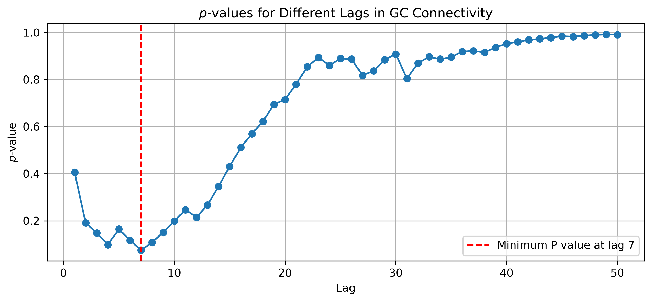
How the best lag is determined using p-values: The plot shows p-values calculated for each lag, with the minimum occurring around lag 7, after which the p-values increase. The algorithm selects this minimum as the best lag.

In one line:

dn.connectivity(ts1, ts2, "gc", lag_steps=max_lag)

(np.float64(0.07471915278791565), 7)

Using Connectivity Measures

delaynet provides a unified interface for all connectivity measures through the connectivity() function. A diverse set of connectivity metrics to analyze relationships between time series data are available. Each metric offers different approaches to detecting connections, from simple correlations to complex causality measures. You can refer to each method by its full name or by its shorthand:

• Granger Causality: Statistical concept of causality based on prediction

  • gc, granger causality, or gt_multi_lag

• Transfer Entropy: Measures the amount of directed transfer of information between two random processes

  • te, transfer entropy, or transfer_entropy

• Mutual Information: Measures the amount of information obtained about one random variable through observing another

  • mi, mutual information, or mutual_information

• Linear Correlation: Calculates the Pearson correlation coefficient between two time series

  • lc, linear correlation, or linear_correlation

• Rank Correlation: Calculates the Spearman rank correlation between two time series

  • rc, rank correlation, or rank_correlation

• Continuous Ordinal Patterns: Analyzes patterns in time series data to detect relationships

  • cop, continuous ordinal patterns, or random_patterns

• Gravity: A toy metric for educational purposes

  • gv, or gravity

import delaynet as dn

# Calculate connectivity between two time series
result = dn.connectivity(ts1, ts2, metric="linear_correlation", lag_steps=5)
# tests all 1, ...., 5 lags
result = dn.connectivity(ts1, ts2, metric="lc", lag_steps=[1, 2, 5, 10])
# tests only specified lags using shorthand

Now, result is a tuple of the best \(p\)-value and the corresponding delay step. For example, if result is (0.05, 3), it means that the best \(p\)-value is 0.05 and it occurs with a lag of 3 time steps.

You can view all available connectivity measures using the show_connectivity_metrics() function:

from delaynet.connectivity import show_connectivity_metrics

# Show all available connectivity measures
show_connectivity_metrics()

Show code cell output

Hide code cell output

Available connectivity metrics:

Metric: random_patterns
Aliases:
 - continuous ordinal patterns
 - cop
 - random_patterns

Metric: gt_multi_lag
Aliases:
 - granger causality
 - gc
 - gt_multi_lag

Metric: gravity
Aliases:
 - gravity
 - gv

Metric: linear_correlation
Aliases:
 - linear correlation
 - lc
 - linear_correlation

Metric: mutual_information
Aliases:
 - mutual information
 - mi
 - mutual_information

Metric: rank_correlation
Aliases:
 - rank correlation
 - rc
 - rank_correlation

Metric: transfer_entropy
Aliases:
 - transfer entropy
 - te
 - transfer_entropy

Analysing the same time series data from the earlier example, switching between connectivity metrics is really simple:

max_lag = 40
(dn.connectivity(ts1, ts2, "gc", lag_steps=max_lag),
dn.connectivity(ts1, ts2, "mi", lag_steps=max_lag, approach="metric"),
dn.connectivity(ts1, ts2, "te", lag_steps=max_lag, approach="metric"),
dn.connectivity(ts1, ts2, "lc", lag_steps=max_lag),
dn.connectivity(ts1, ts2, "rc", lag_steps=max_lag),
dn.connectivity(ts1, ts2, "cop", lag_steps=max_lag),
dn.connectivity(ts1, ts2, "gv", lag_steps=max_lag))

((np.float64(0.07471915278791565), 7),
 (np.float64(0.0), 2),
 (np.float64(0.0), 5),
 (np.float64(0.058758562650754326), 31),
 (np.float64(0.012092430710742176), 31),
 (np.float64(0.01584687475460676), 1),
 (np.float64(0.0), 5))

For some connectivity measures the optimal lags agree with each other, but they generally vary, especially the p-values, as each of these approaches covers a different type of connectivity.

For details about these connectivity methods, see the next subsections.