Preparation

This section covers the data preparation functionality in delaynet. First, Data preparation describes what input data delaynet needs. Second, Data generation will describe how to generate synthetic data for testing and experimentation.

Data preparation

In order to reconstruct delay functional networks, delaynet requires a set of time series data for each node in the network. For each pair of nodes a weight as \(p\)-value can be calculated with a given connectivity measure. The data length must be consistent across all nodes. For example, having ten nodes with time series:

Show code cell source

Hide code cell source

import pandas as pd
import numpy as np

# randomly generated columns
nodes = 10
ts_len = 200
# do random walks for each node
data = np.random.randint(low=-1, high=2, size=(ts_len, nodes))
# running culmulate (1d random walks)
data = np.cumsum(data, axis=0)

data = pd.DataFrame(
    index=pd.date_range(start=pd.Timestamp.now().floor('h'), periods=ts_len, freq='10min'),
    columns=range(1, nodes+1),
    data=data,
)
data

	1	2	3	4	5	6	7	8	9	10
2026-04-14 08:00:00	0	-1	0	-1	1	1	0	0	0	-1
2026-04-14 08:10:00	-1	-1	0	-1	0	1	0	1	0	-2
2026-04-14 08:20:00	-2	0	0	0	1	2	-1	1	1	-3
2026-04-14 08:30:00	-1	-1	1	0	2	2	-1	1	0	-3
2026-04-14 08:40:00	-1	0	0	-1	2	3	0	0	1	-2
...	...	...	...	...	...	...	...	...	...	...
2026-04-15 16:30:00	-12	6	-5	-4	5	18	-9	-9	-11	1
2026-04-15 16:40:00	-12	7	-4	-4	4	19	-8	-9	-12	2
2026-04-15 16:50:00	-12	6	-4	-5	4	18	-8	-9	-11	3
2026-04-15 17:00:00	-11	5	-3	-4	4	19	-8	-10	-10	3
2026-04-15 17:10:00	-11	5	-3	-5	5	19	-8	-10	-11	4

200 rows × 10 columns

Data cleaning

Before performing any detrending and connectivity analysis, it’s crucial to clean the data. This includes handling missing values and outliers.

Attention

When working with time series data, it’s important to check for NaN values and missing data before analysis. delaynet currently doesn’t provide specific functions for handling NaN values or missing data. When preprocessing your data, make sure you choose a method that best suits your dataset and research question, e.g. replacing NaNs with zeros, mean, median imputation, or using interpolation methods.

Handling Missing Values

Missing values can be handled by filling them with a specific value or method like mean imputation:

import numpy as np

# Sample data with missing values
data = np.array([10.0, 20.0, None, np.nan, 50.0], dtype=np.float64)

# Fill missing values - in-place replacement
np.nan_to_num(data, nan=0.0, copy=False)
data

array([10., 20.,  0.,  0., 50.])

If you already have a dataset, you can advance to the next section.

Data generation

delaynet provides several methods for generating synthetic data that can be used for testing and experimentation. The library offers two primary data generation methods:

1. Delayed Causal Network Generation: Creates time series with explicit causal relationships and time delays between nodes, suitable for testing delay network reconstruction algorithms.

2. fMRI Data Generation: Simulates realistic fMRI signals with haemodynamic response functions, based on neuroimaging research.

3. SynthATDelays Transportation Delay Generation: Generates realistic transportation delay data through integration with the specialised simulation tool SynthATDelays, offering controlled scenarios for testing delay propagation in transportation networks.

Each method provides specific functions for generating different types of synthetic data:

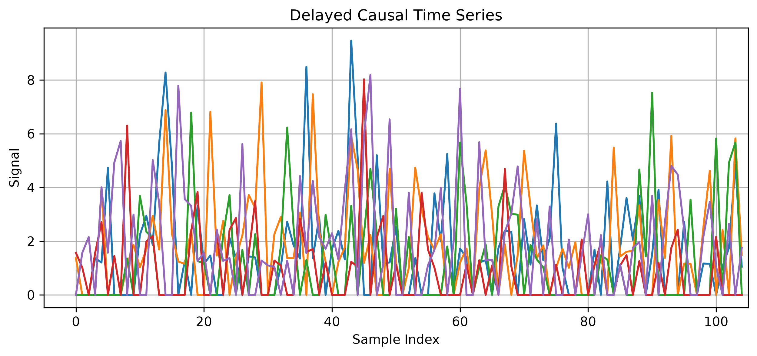
1. Delayed Causal Network Generation

The delayed causal network generation process follows these steps:

1. Adjacency Matrix Generation: Creates a random binary matrix where each entry has a probability l_dens of being 1 (indicating a connection). Self-loops are explicitly removed by setting diagonal elements to False.

2. Weight Matrix Creation: Assigns random weights to connections in the adjacency matrix. Weights are uniformly distributed between the minimum and maximum values specified in wm_min_max. Non-connections (where adjacency matrix is 0) have zero weight.

3. Lag Matrix Generation: Creates a matrix of random integers between 1 and 4, representing time delays between connected nodes.

4. Time Series Generation: For each connection in the network:

   • With 80% probability, no effect is applied (simulating sporadic influence)

   • With 20% probability, a value from an exponential distribution is generated, scaled by the connection weight

   • This value is added to the source node’s time series

   • The same value is added to the target node’s time series after the specified lag

This approach creates time series with causal relationships that have both magnitude ( weight) and temporal (lag) components, making it suitable for testing delay network reconstruction algorithms.

import delaynet as dn
from numpy.random import default_rng

# Generate random data
adjacency_matrix, weight_matrix, time_series = dn.preparation.data_generator.gen_delayed_causal_network(
    ts_len=1000,  # Length of time series
    n_nodes=5,    # Number of nodes
    l_dens=0.3,   # Density of the adjacency matrix
    wm_min_max=(0.5, 1.5),  # Min and max of the weight matrix
    rng=default_rng(1249687)
)

Show code cell source

Hide code cell source

import matplotlib.pyplot as plt

# Plot the time series data
plt.figure(figsize=(10, 4), dpi=300)
plt.plot(time_series.T[:105])
plt.title('Delayed Causal Time Series')
plt.xlim(-5, 105)
plt.xlabel('Sample Index')
plt.ylabel('Signal')
plt.grid()
plt.show()

2. fMRI Data Generation

The functional Magnetic Resonance Imaging (fMRI) data generation process simulates realistic functional MRI signals by modeling both the underlying neural activity and the haemodynamic response. This approach is based on studies by Roebroeck et al. and Rajapakse and Zhou [RZ07, RFG05].

Roebroeck et al. [RFG05] proposed Granger causality mapping (GCM) as an approach to explore directed influences between neuronal populations in fMRI data. Their method doesn’t rely on a priori specification of a model with pre-selected regions and connections, instead using temporal precedence information to identify voxels that are sources or targets of directed influence. Rajapakse and Zhou [RZ07] extended this work by using dynamic Bayesian networks (DBN) to learn effective brain connectivity. Their approach uses a Markov chain to model fMRI time-series and determine temporal relationships between brain regions. Their research demonstrated that DBN performance is comparable to GCM for linearly connected networks, while providing more complete statistical descriptions of connectivity. They also studied the effects of various noise types, inter-scan intervals, and haemodynamic parameter variability on connectivity analysis. Together, these papers provide the theoretical foundation for generating realistic fMRI data with directed causal influences.

The generation process follows these steps:

1. Initial Time Series Generation: Creates coupled time series representing underlying neural activity:

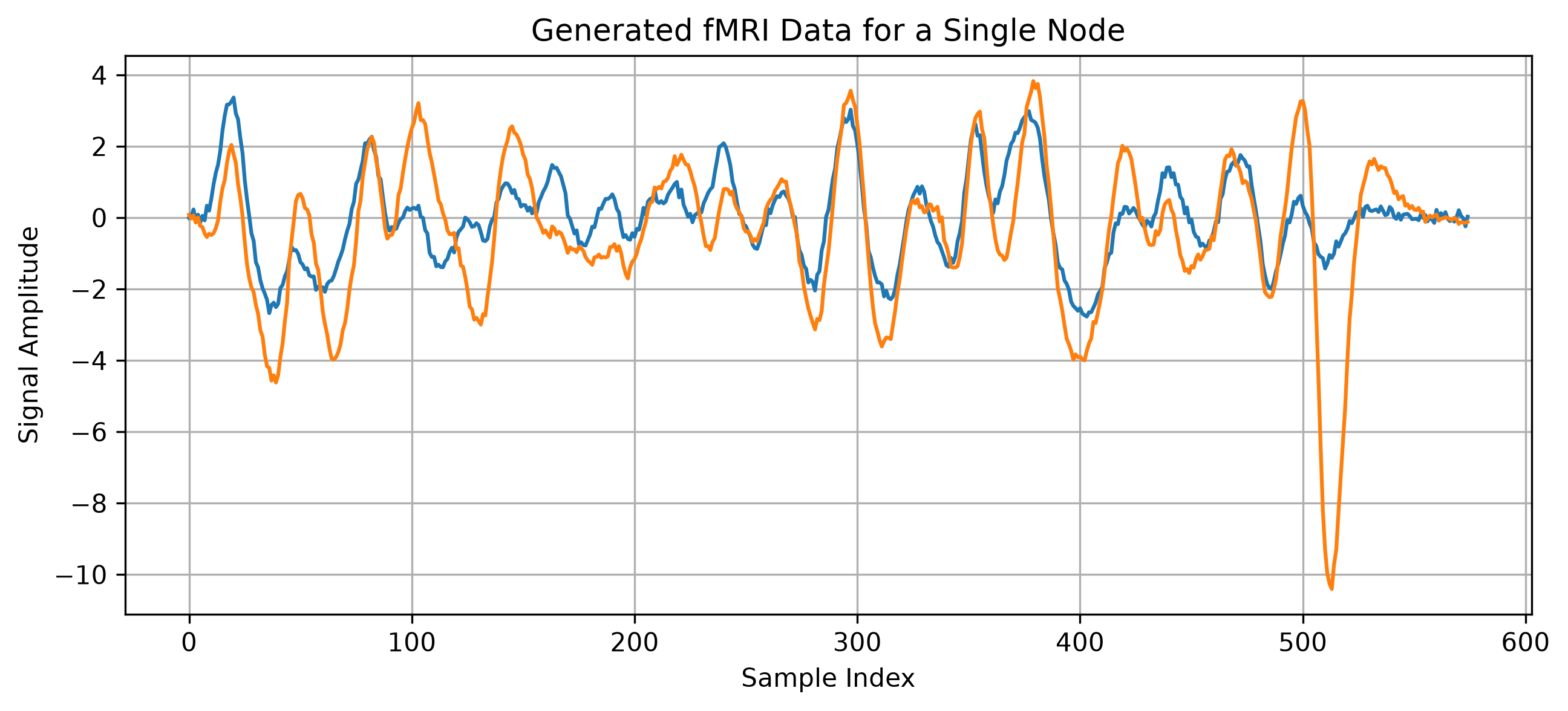
   • For a single node gen_fmri(): Generates two coupled time series with specified coupling strength

   • For multiple nodes gen_fmri_multiple(): Creates a network where the first node influences all other nodes with the specified coupling strength

2. Hemodynamic Response Function (HRF) Application: Convolves the neural activity with a haemodynamic response function:

   • The HRF is modeled using gamma distributions with both peak and undershoot components

   • This simulates the blood-oxygen-level-dependent (BOLD) response that fMRI measures

3. Downsampling: Reduces the temporal resolution of the signal to match typical fMRI acquisition rates:

   • The downsampling factor parameter controls the temporal resolution

   • This simulates the relatively slow sampling rate of fMRI compared to actual neural activity

4. Noise Addition: Adds Gaussian noise to the final time series:

   • The noise level can be controlled separately for the initial neural activity and the final fMRI signal

   • This simulates measurement noise in real fMRI data

This approach creates a realistic fMRI time series with directed influences between regions, making it suitable for testing connectivity analysis methods in neuroimaging research.

# Generate fMRI data for a single node
fmri_data = dn.preparation.data_generator.gen_fmri(
    ts_len=1000,               # Length of time series
    downsampling_factor=2,     # Downsampling factor
    time_resolution=0.2,       # Time resolution
    coupling_strength=2.0,     # Coupling strength
    noise_initial_sd=1.0,      # Standard deviation of initial noise
    noise_final_sd=0.1,        # Standard deviation of final noise
    rng=default_rng(1249687)
)

Show code cell source

Hide code cell source

# Plot the generated fMRI data for a single node
plt.figure(figsize=(10, 4), dpi=300)
plt.plot(fmri_data)
plt.title('Generated fMRI Data for a Single Node')
plt.xlabel('Sample Index')
plt.ylabel('Signal Amplitude')
plt.grid()
plt.show()

# Generate fMRI data for multiple nodes
multi_fmri_data = dn.preparation.data_generator.gen_fmri_multiple(
    ts_len=1000,               # Length of time series
    n_nodes=5,                 # Number of nodes
    downsampling_factor=2,     # Downsampling factor
    time_resolution=0.2,       # Time resolution
    coupling_strength=2.0,     # Coupling strength
    noise_initial_sd=1.0,      # Standard deviation of initial noise
    noise_final_sd=0.1,        # Standard deviation of final noise
    rng=default_rng(1249687)
)

Show code cell source

Hide code cell source

# Plot multiple nodes' fMRI data
plt.figure(figsize=(12, 6), dpi=300)
plt.plot(multi_fmri_data.T, label=range(1, multi_fmri_data.shape[0]+1))
plt.xlabel('Sample Index')
plt.ylabel('Signal Amplitude')
plt.title('Generated FMRI Data for Multiple Nodes')
plt.legend()
plt.grid()
plt.show()

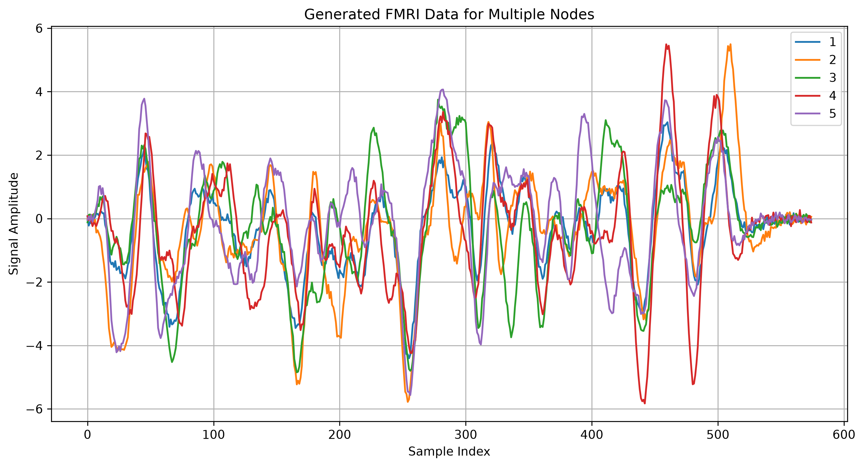
The generated fMRI data simulates realistic brain activity patterns with directed influences between regions, making it suitable for testing connectivity analysis methods.

3. SynthATDelays Transportation Delay Generation

The SynthATDelays transportation delay generation process creates realistic delay data specifically designed for transportation networks. This approach addresses a critical limitation in delay dynamics analysis—the impossibility of executing what-if scenarios with real systems. Unlike comprehensive air transport simulators that aim for maximum realism at high computational cost, this method focuses on generating highly tunable scenarios to test specific conditions and hypotheses. This integration offers two predefined scenarios, but more intricate scenarios can be simulated, when using all the features of SynthATDelays. For this, visit their documentation. The predefined scenarios are:

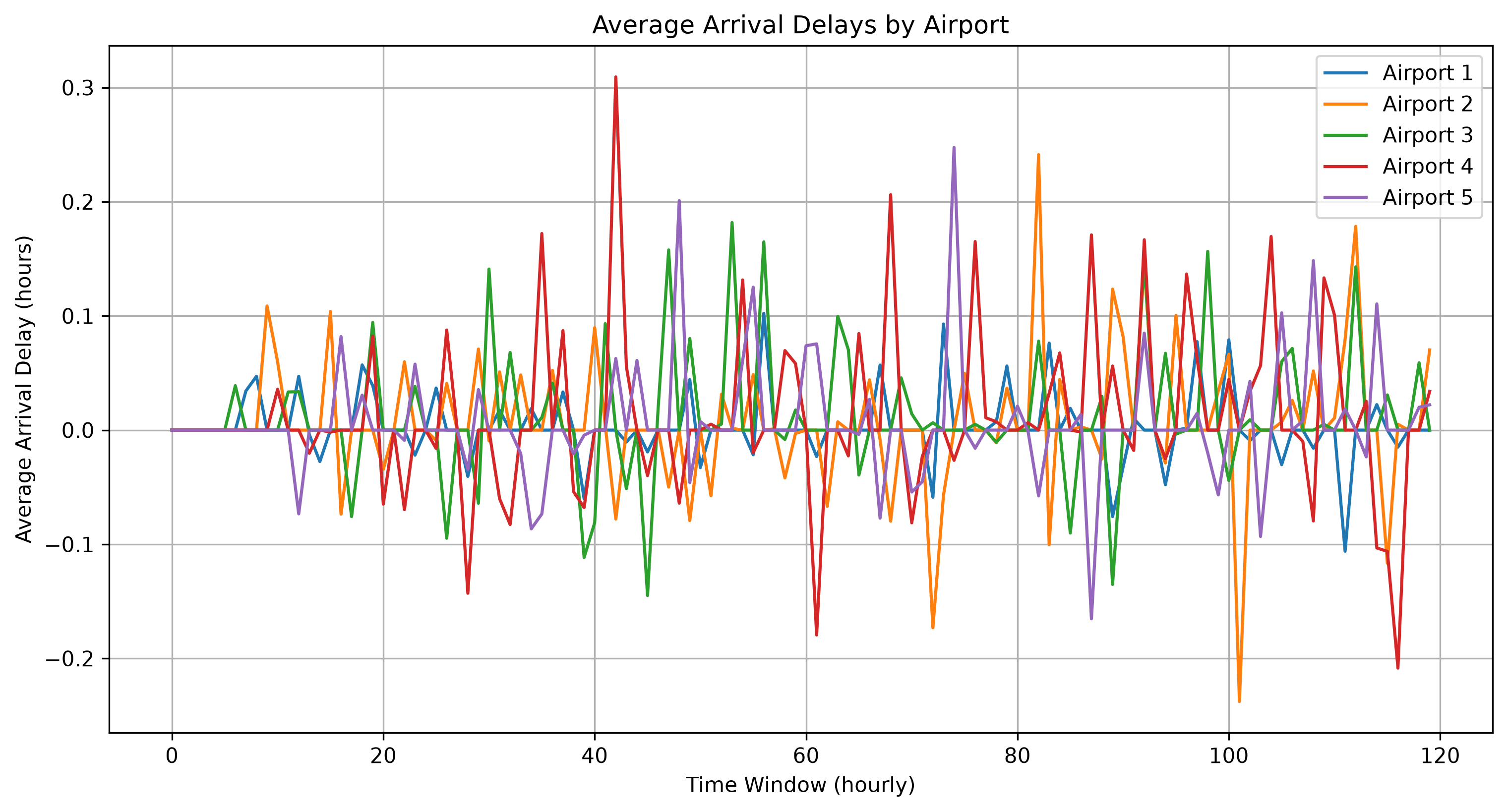
Random Connectivity Scenario

This scenario simulates a set of airports randomly connected by independent flights, with random and homogeneous enroute delays. It allows customisation of:

• Number of airports

• Number of aircraft

• Buffer time between operations

# Generate delay data using the Random Connectivity scenario
from delaynet.preparation import gen_synthatdelays_random_connectivity

results = gen_synthatdelays_random_connectivity(
    sim_time=5,               # Simulation time in days
    num_airports=5,           # Number of airports
    num_aircraft=10,          # Number of aircraft
    buffer_time=0.8,          # Buffer time between operations in hours
    seed=42                   # Random seed for reproducibility
)

# Extract the average arrival delay matrix
arrival_delays = results.avgArrivalDelay
print(f"Shape of arrival delays matrix: {arrival_delays.shape}")

Shape of arrival delays matrix: (120, 5)

# Plot the average arrival delays for each airport
plt.figure(figsize=(12, 6), dpi=300)
for i in range(arrival_delays.shape[1]):
    plt.plot(arrival_delays[:, i], label=f"Airport {i+1}")
plt.xlabel("Time Window (hourly)")
plt.ylabel("Average Arrival Delay (hours)")
plt.title("Average Arrival Delays by Airport")
plt.legend()
plt.grid()
plt.show()

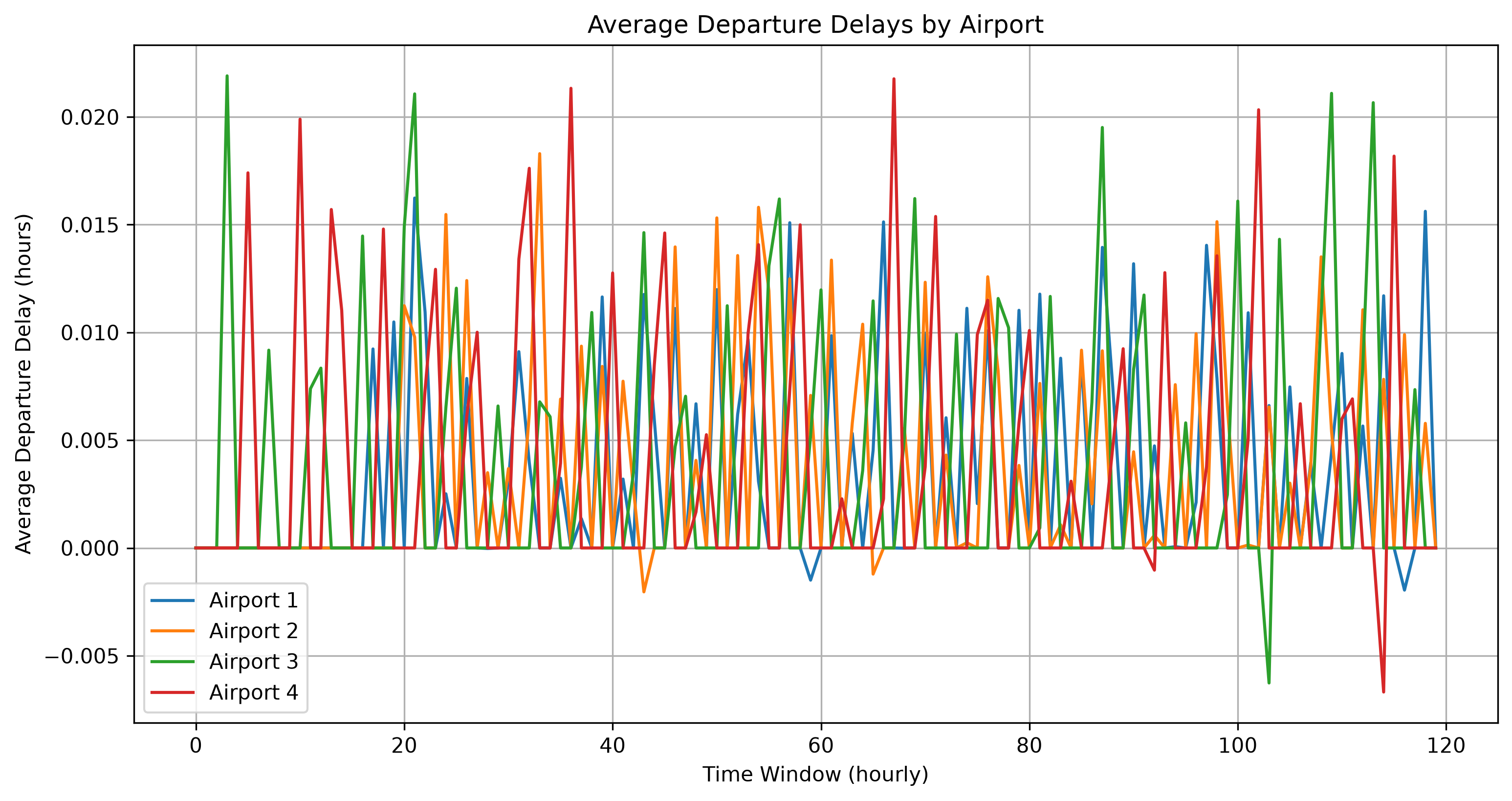
Independent Operations with Trends Scenario

This scenario creates two groups of two airports, where flights connect airports within the same group but not across groups. When trends are activated, delays are added at specific hours, generating spurious causality relations between airports despite no actual propagation pathways between groups.

# Generate delay data using the Independent Operations with Trends scenario
from delaynet.preparation import gen_synthatdelays_independent_operations_with_trends

results = gen_synthatdelays_independent_operations_with_trends(
    sim_time=5,               # Simulation time in days
    activate_trend=True,      # Activate trends at specific hours
    seed=42                   # Random seed for reproducibility
)

# Extract the average departure delay matrix
departure_delays = results.avgDepartureDelay
print(f"Shape of departure delays matrix: {departure_delays.shape}")

Shape of departure delays matrix: (120, 4)

# Plot the average departure delays for each airport
plt.figure(figsize=(12, 6), dpi=300)
for i in range(departure_delays.shape[1]):
    plt.plot(departure_delays[:, i], label=f"Airport {i+1}")
plt.xlabel("Time Window (hourly)")
plt.ylabel("Average Departure Delay (hours)")
plt.title("Average Departure Delays by Airport")
plt.legend()
plt.grid()
plt.show()

Working with SynthATDelays Results

The SynthATDelays generators return a Results_Class object containing various delay metrics. To extract specific delay time series, you can use the helper function:

# Extract delay time series from results
from delaynet.preparation import extract_airport_delay_time_series

# Get arrival delays
arrival_delays = extract_airport_delay_time_series(results, "arrival")

# Get departure delays
departure_delays = extract_airport_delay_time_series(results, "departure")

These synthetic transportation delay datasets enable researchers to validate analytical methods, benchmark connectivity measures, and explore specific propagation scenarios under controlled conditions. This is particularly valuable in transportation research where ground truth propagation patterns are often challenging to establish from observational data alone.