
Network Analysis#
Network analysis involves studying the structural properties of networks to understand
their organization, robustness, and function. This analysis can reveal important
features such as centrality of nodes, network efficiency, and connection patterns. The
delaynet package provides a set of tools for analyzing reconstructed networks,
including functions for pruning networks and calculating various network metrics.
This guide demonstrates how to use the network analysis functionality in delaynet to
extract meaningful insights from reconstructed networks.
Network Pruning#
Network pruning is the process of simplifying a complex network by removing weak or insignificant connections. This is an important step in network analysis as it helps to focus on the most important relationships and reduce noise. This can also support science communication by highlighting the most important relationships in a network.
As described in the Network Reconstruction section, the weight matrix in network reconstruction represents a matrix of \(p\)-values, where lower values indicate stronger connections. Network pruning methods typically remove connections with \(p\)-values above a certain threshold, retaining only the strongest and most significant connections.
Statistical Pruning#
The delaynet package provides the
statistical_pruning() function for pruning
networks
based on statistical significance. This function takes a matrix of \(p\)-values and
returns a boolean mask indicating which connections are statistically significant.
For this example, we are using the same network as from the previous page, but with an
added node with random data.
import numpy as np
import matplotlib.pyplot as plt
import networkx as nx
import delaynet as dn
from numpy.random import default_rng

# Generate synthetic data
adjacency_matrix, weight_matrix, time_series = dn.preparation.gen_delayed_causal_network(
    ts_len=1000,                # Length of time series
    n_nodes=8,                  # Number of nodes
    l_dens=0.5,                 # Density of the adjacency matrix
    wm_min_max=(0.5, 1.5),      # Min and max of the weight matrix
    rng=default_rng(1612757)
)

# Add random row to time series - to demonstrate separated node
random_data = np.random.default_rng(3465).standard_normal(time_series.shape[1])
time_series = np.vstack((time_series, random_data))

# Detrend the time series
time_series = dn.detrend(time_series, "delta", axis=1)

# Reconstruct the network
weights, lags = dn.reconstruct_network(
    time_series.T, connectivity_measure="gc", lag_steps=10
)

print(f"Shape of p-value matrix: {weights.shape}")
print(f"Shape of lag matrix: {lags.shape}")
Sequential: [##############################] 72/72 (100.0%) Time: 1.0s
Shape of p-value matrix: (9, 9)
Shape of lag matrix: (9, 9)
Now that we have reconstructed the network, we can visualize the p-value matrix:
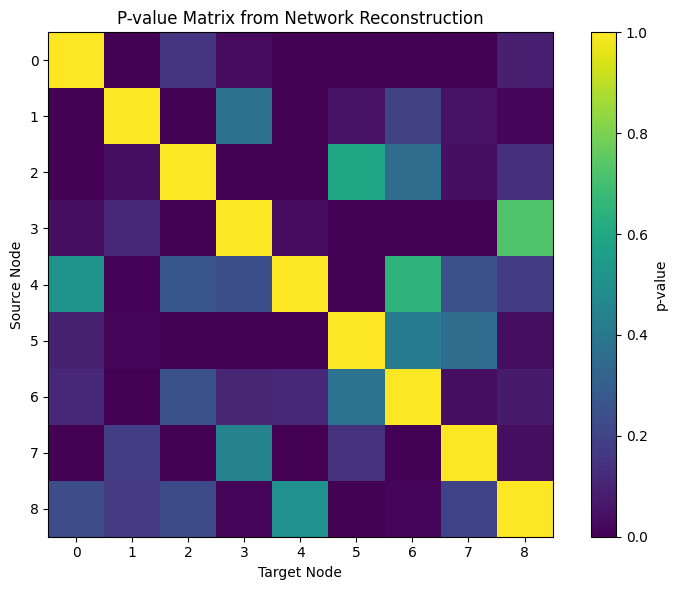
Lower p-values (darker colors) indicate stronger connections between nodes. To focus on the most significant connections, we can apply statistical pruning:
# Apply statistical pruning with a significance level of 0.05
# and Benjamini-Hochberg false discovery rate correction
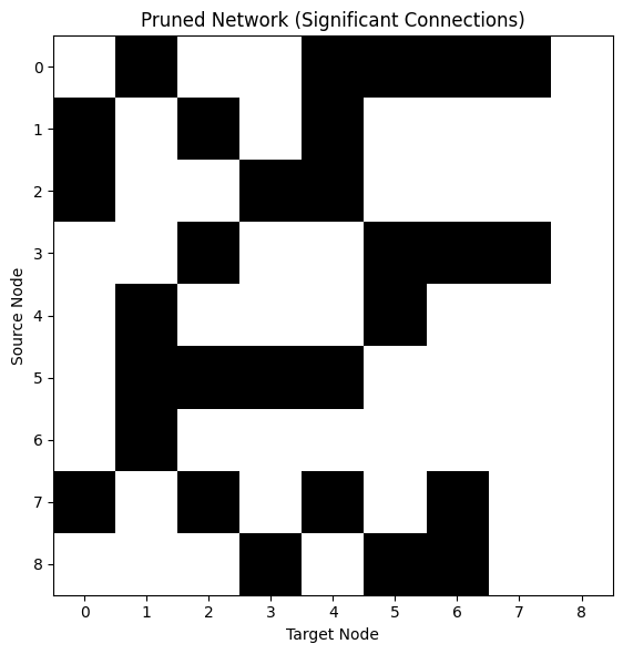
significant_connections = dn.network_analysis.statistical_pruning(
weights, alpha=0.05, correction='fdr_bh'
)
print(f"Shape of pruned matrix: {significant_connections.shape}")
print(f"Number of significant connections: {np.sum(significant_connections)}")
Shape of pruned matrix: (9, 9)
Number of significant connections: 29
The pruning function returns a boolean mask where True indicates a significant
connection. We can visualize this pruned network:
Multiple Comparison Correction
When testing multiple connections simultaneously, the chance of finding at least one significant result by random chance increases with the number of tests. The statistical_pruning() function supports any correction method available in statsmodels.stats.multitest.multipletests(). Common methods include:
‘bonferroni’: Conservative correction that controls the family-wise error rate
‘holm’: Step-down method using Bonferroni adjustments
‘fdr_bh’: Benjamini-Hochberg procedure to control the false discovery rate
‘fdr_by’: Benjamini-Yekutieli procedure for dependent tests
Additional available methods include:
‘sidak’: Šidák correction (less conservative than Bonferroni)
‘holm-sidak’: Step-down method using Šidák adjustments
‘hommel’: Closed method based on Simes tests (non-negative)
‘fdr_tsbh’: Two-stage FDR correction (Benjamini-Hochberg)
Choose the appropriate correction method based on your specific requirements, the characteristics of your data, and whether your tests can be assumed to be independent.
Network Metrics#
Once we have a pruned network, we can calculate various metrics to analyze its
properties. The delaynet.network_analysis module provides several functions for
calculating network metrics.
Before diving into the calculation of network metrics, it’s important to understand what
each metric represents and how it can be interpreted in the context of transportation
networks.
Link Density#
link_density() quantifies how densely connected
a network is by calculating the proportion of actual connections relative to the maximum
possible connections.
For a network with \(n\) nodes, link density is calculated as:
Directed networks: \(\text{density} = \frac{E}{n(n-1)}\)
Undirected networks: \(\text{density} = \frac{2E}{n(n-1)}\)
where \(E\) is the number of edges (connections) in the network. Values range from 0 (no connections) to 1 (fully connected) where higher values indicate more densely connected networks. In transportation networks, higher density often suggests more redundant pathways and potentially more resilience to disruptions. As we measure delay propagation, this “efficiency” is regarding delays propagating. A transport network resilient to delay propagation must be characterised by a lower global efficiency for the delay propagation network.
# Convert boolean mask to binary adjacency matrix
binary_adjacency = significant_connections.astype(int)

# Calculate link density
density = dn.network_analysis.link_density(binary_adjacency)
print(f"Link density: {density:.4f}")
Link density: 0.4028
Isolated Nodes#
These metrics identify nodes that are disconnected from the rest of the network in terms
of incoming or outgoing connections.
Nodes with no incoming connections
isolated_nodes_inbound() don’t receive delays
from
other nodes.
Nodes with no outgoing connections
isolated_nodes_outbound() don’t propagate
delays to
other nodes.
In transportation networks, isolated nodes may represent stations or airports that
operate independently of the broader network.
# Find isolated nodes
isolated_in = dn.network_analysis.isolated_nodes_inbound(binary_adjacency)
isolated_out = dn.network_analysis.isolated_nodes_outbound(binary_adjacency)

print(f"Nodes with no incoming connections: {isolated_in}")
print(f"Nodes with no outgoing connections: {isolated_out}")
Nodes with no incoming connections: 1
Nodes with no outgoing connections: 0
Centrality Measures#
Centrality measures help identify the most important or influential nodes in a network:
Betweenness Centrality#
betweenness_centrality() is a prominent measure
of centrality which tries to measure the importance of a node or edge in a network by
counting the number of shortest paths that lead through it
[Bra08].
Nodes with high betweenness centrality act as bridges or bottlenecks in the network.
These nodes control information flow between different parts of the network.
In transportation networks, high betweenness nodes are critical junctions where many
routes pass through.
Disruptions at these nodes can have widespread effects throughout the network.
For delay networks, high betweenness nodes can be nodes that hand through delays.
Eigenvector Centrality#
eigenvector_centrality() measures a node’s
influence based on the principle that connections to high-scoring nodes contribute more
to the score than connections to low-scoring nodes.
Nodes with high eigenvector centrality are connected to other important nodes.
This metric captures the concept that “importance” is recursive - a node is important if
it’s connected to other important nodes.
In transportation networks, high eigenvector centrality may identify hubs that connect
to other major hubs.
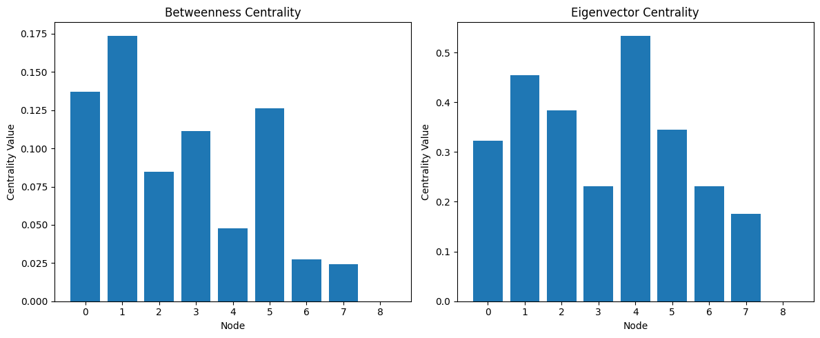
# Calculate betweenness centrality
betweenness = dn.network_analysis.betweenness_centrality(binary_adjacency)
print(f"Betweenness centrality: {betweenness}")

# Calculate eigenvector centrality
eigenvector = dn.network_analysis.eigenvector_centrality(binary_adjacency)
print(f"Eigenvector centrality: {eigenvector}")
Betweenness centrality: [0.13690476 0.17380952 0.08452381 0.11130952 0.04761905 0.12619048
 0.02738095 0.02440476 0.        ]
Eigenvector centrality: [ 0.32202145  0.45496602  0.3833937   0.2313868   0.53391971  0.3452771
  0.23153613  0.17573281 -0.        ]
Let’s visualize these centrality measures:
Global Efficiency#
global_efficiency() quantifies how efficiently
information can flow through the network, calculated as the average of the inverse
shortest path lengths between all pairs of nodes
[LM01].
Values range from 0 (completely disconnected) to 1 (perfectly efficient), where higher
values indicate more efficient networks with shorter paths between nodes.
In transportation networks, higher efficiency suggests better connectivity and
potentially faster travel times.
Networks with high global efficiency are often more resilient to random failures but may
be vulnerable to targeted attacks on high-centrality nodes.
# Calculate global efficiency
efficiency = dn.network_analysis.global_efficiency(binary_adjacency)
print(f"Global efficiency: {efficiency:.4f}")
Global efficiency: 0.6319
Transitivity (Clustering Coefficient)#
transitivity() measures the tendency of the
network to form clusters, calculated as the fraction of all possible triangles present
in the graph.
Values range from 0 (no clustering) to 1 (fully clustered), where higher values indicate
more clustering, where neighbors of a node tend to be connected to each other.
In transportation networks, high transitivity may indicate regional clusters with good
local connectivity.
Networks with high transitivity often have redundant paths within clusters but may have
bottlenecks between clusters.
Note that transitivity is defined for undirected graphs. For directed networks, the direction of edges is ignored when calculating transitivity, as the concept of triangles is defined for undirected graphs. For directed networks, consider using reciprocity (see below) to measure the tendency of vertex pairs to form mutual connections.
# Calculate transitivity
trans = dn.network_analysis.transitivity(binary_adjacency)
print(f"Transitivity: {trans:.4f}")
Transitivity: 0.6122
Reciprocity#
reciprocity() measures the tendency of vertex
pairs to form mutual connections in a directed network. It is defined as the fraction of
edges that are reciprocated.
Formally, the reciprocity is calculated as:
where \(m\) is the number of edges and \(A\) is the adjacency matrix of the graph. Note that \(A_{i,j} A_{j,i} = 1\) if and only if \(i\) links to \(j\) and vice versa. Values range from 0 (no reciprocated edges) to 1 (all edges are reciprocated). In transportation networks, high reciprocity may indicate bidirectional routes or mutual dependencies between locations. Reciprocity is only defined for directed networks. For undirected networks, all connections are reciprocal by definition.
# Calculate reciprocity (only for directed networks)
recip = dn.network_analysis.reciprocity(binary_adjacency)
print(f"Reciprocity: {recip:.4f}")
Reciprocity: 0.4138
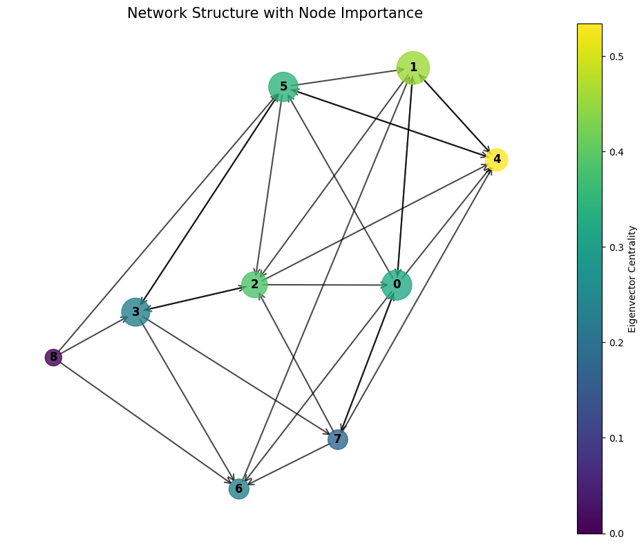
Network Visualization#
We can visualize the network using NetworkX to better understand its structure:
Working with Weighted Networks
All network analysis functions in delaynet can work with both binary and weighted networks. For weighted networks:
The weight matrix should contain positive values representing connection strengths
The
directedparameter can be set toTrueorFalsedepending on whether the network is directed or undirectedSome metrics, like betweenness centrality, interpret weights as distances, so stronger connections should have higher values
When working with p-values from network reconstruction, you may want to transform them (e.g., -log10(p_values)) to use them as weights, since lower p-values indicate stronger connections.
Understanding Network Analysis Results#
The metrics used in transportation network analysis provide valuable insights into network structure, efficiency, and vulnerability. Understanding how to interpret these results is crucial for making informed decisions about network management and development.
In transportation networks, critical nodes are points whose disruption would significantly impact overall network performance. These can be identified in several ways. Nodes with high betweenness centrality typically represent critical junctions or transfer points, such as major train stations, airport hubs, or highway intersections. These are locations where many shortest paths converge. Similarly, nodes with high eigenvector centrality are usually well-connected to other important nodes, often forming major hubs that connect to other hubs and create the backbone of the network. Additionally, nodes that would significantly decrease global efficiency if removed are considered critical for maintaining efficient operations across the network.
Network resilience, which describes a network’s ability to maintain functionality during disruptions, can be assessed through several characteristics. A high link density typically suggests the presence of redundant pathways, offering alternative routes when disruptions occur. High transitivity or clustering indicates good local connectivity, which helps contain the impact of disruptions within specific regions. However, it’s important to maintain a balance between efficiency and redundancy, as highly efficient networks with minimal redundancy may become vulnerable to targeted disruptions.
Communities within transportation networks typically manifest as regional clusters with strong internal connectivity. These can be identified through various indicators. Areas showing high transitivity often represent community structures where nodes are densely connected within groups. Between these communities, bottlenecks can be identified by nodes with high betweenness centrality that serve as connections between different clusters. While not directly implemented in delaynet, community detection algorithms available in libraries like NetworkX or igraph can formally identify these structures.
When examining how networks evolve over time or comparing different networks, several patterns may emerge. Changes in centrality measures often indicate shifting importance of different nodes within the network. An increase in global efficiency might point to infrastructure improvements or optimization efforts. Meanwhile, changes in transitivity could suggest evolving community structures or regional development patterns. These temporal comparisons provide valuable insights into network evolution and development trends.
Comparing Networks#
Network metrics can be used to compare different networks or the same network under different conditions:
# Generate a random network with the same number of nodes and edges
random_network = np.random.random(binary_adjacency.shape) < density
random_network = random_network.astype(int)

# Calculate metrics for both networks
metrics_original = {
    'density': dn.network_analysis.link_density(binary_adjacency),
    'efficiency': dn.network_analysis.global_efficiency(binary_adjacency),
    'transitivity': dn.network_analysis.transitivity(binary_adjacency)
}

metrics_random = {
    'density': dn.network_analysis.link_density(random_network),
    'efficiency': dn.network_analysis.global_efficiency(random_network),
    'transitivity': dn.network_analysis.transitivity(random_network)
}

# Print comparison
print("Comparison of network metrics:")
for metric in metrics_original:
    print(f"{metric.capitalize()}:")
    print(f"  Original network: {metrics_original[metric]:.4f}")
    print(f"  Random network:   {metrics_random[metric]:.4f}")
Comparison of network metrics:
Density:
  Original network: 0.4028
  Random network:   0.3611
Efficiency:
  Original network: 0.6319
  Random network:   0.6389
Transitivity:
  Original network: 0.6122
  Random network:   0.6000
If you are interested in applications of these metrics and reconstruction examples, the next demonstrates a few applied examples.